A route to more fully understanding ITM has been using it to recreate graphs in the 1982 "Guide to the Use of the ITS Irregular Terrain Model in the Area Prediction Mode." Several small programs written to do so are provided below. Graphed results are overlaid on the originals for easy comparison.
The program lr.py is mentioned on the main page. Here, we use it to recreate Figure 5 in Section 7.1 in the Area report. It is run by typing:
lr.py < mobile.lr
resulting in output matching Figure 5:
$ lr.py < mobile.lr
   Operational Ranges for a Mobile-to-Mobile System

            Frequency      45.000 MHz
      Antenna heights     2.0     2.0 m
    Effective heights     2.0     2.0 m  (siting=r,r)
     Terrain, delta H          90 m

   Polarity=v, epsilon=15, sigma=0.005 S/m
   Climate=4, N0=301, Ns=301, K=1.333

   First-try success service

   Estimated Quantiles of Basic Transmission Loss (dB)

       Dist     Free    With Confidence
        km     Space     95.0    90.0    80.0    70.0    50.0    20.0    10.0
       ----    -----    -----   -----   -----   -----   -----   -----   -----
        1.0     65.5    113.4   109.7   105.2   102.1    96.9    88.5    84.1
        2.0     71.5    123.0   119.2   114.8   111.6   106.4    97.9    93.5
        3.0     75.1    128.8   125.0   120.5   117.3   112.0   103.6    99.1
        4.0     77.6    133.1   129.2   124.7   121.5   116.2   107.7   103.1
        5.0     79.5    136.4   132.6   128.0   124.8   119.5   110.9   106.3
        6.0     81.1    139.3   135.4   130.8   127.6   122.2   113.6   109.0
        7.0     82.4    141.7   137.8   133.2   130.0   124.6   116.0   111.3
        8.0     83.6    143.9   140.0   135.4   132.1   126.7   118.0   113.4
        9.0     84.6    145.9   141.9   137.3   134.0   128.6   119.9   115.2
       10.0     85.5    147.7   143.7   139.1   135.7   130.3   121.6   116.9
       15.0     89.0    153.4   149.4   144.7   141.4   135.9   127.0   122.3
       20.0     91.5    157.2   153.2   148.4   145.0   139.5   130.6   125.8
       25.0     93.5    160.4   156.3   151.5   148.1   142.6   133.6   128.8
       30.0     95.1    163.2   159.1   154.3   150.8   145.3   136.3   131.4
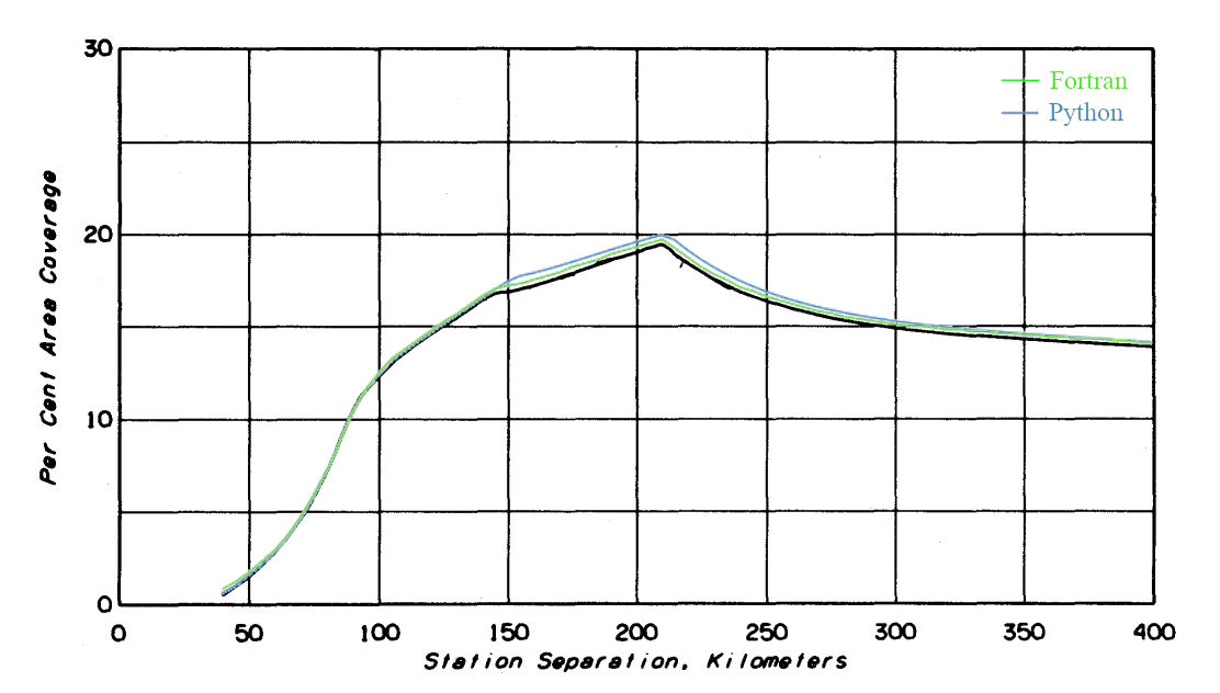
tv.py (7 Jul 2023) makes full use of ITM's variability statistics for television broadcast antenna placement while considering effects of interference. The program solves the problem presented in section 7.2 of the report and is run without command line arguments. A Fortran version, tv.f, was written that links with NTIA's Fortran v1.2.2 ITM for direct comparison. The graph below shows three data sets: results from NTIA's ITM v.1.2.1 in black, NTIA's Fortran v1.2.2 in green, and python v1.2.2 in blue. Max coverages for each are, respectively, 19.5%, 19.6%, and 19.9%. The newer Fortran floats slightly higher than v1.2.1, and python with its fewer approximations slightly higher still, though both v1.2.2 curves coincide asymptotically.
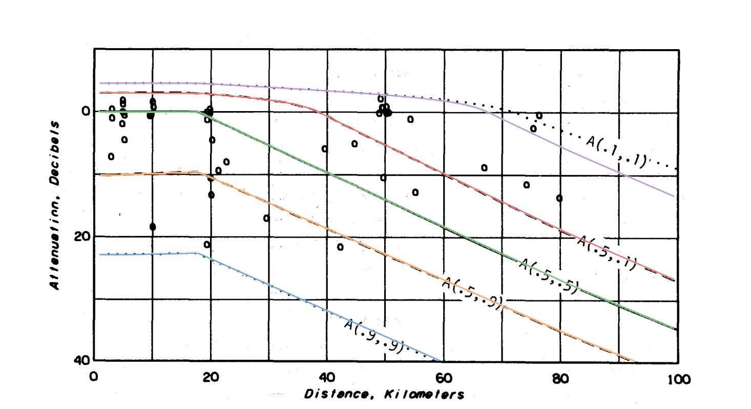
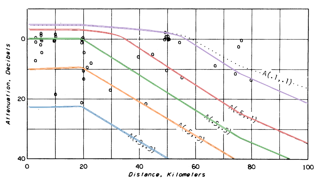
r3.py (13 Jun 2023) runs the model five times to generate the curves of Figure 9 in section 7.3 of the report where stations are sited as 'random.' New colored curves are overlaid on the original black ones. All match extremely well except for A(0.1, 0.1) mode results.
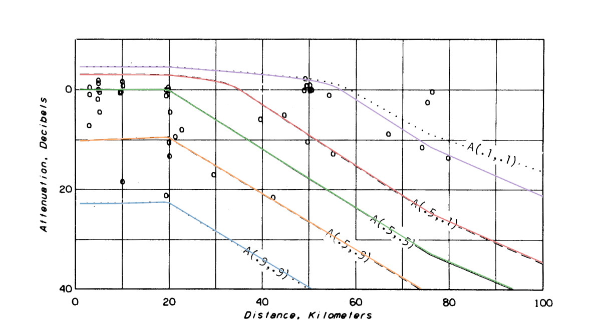
Exploring the A(0.1,0.1) mismatch, I wrote a Fortran version, r3.f of r3.py that links with the NTIA/ITS Fortran v1.2.2 ITM. There are three sets of output on the graph below. Two curves as above, i.e., original report and those based on itm.py, and a third set, output from ITS's Fortran v1.2.2 and r3.f. There are exceedingly slight differences between python and Fortan output as seen below, due in some part to the small numerical differences in Fortran and python implementations and also in some part to the manual process of scaling and overlaying graphs. But both show the marked difference with the 1982 report's A(0.1,0.1). The changes that bring v1.2.1 to v1.2.2 are described as updates to subroutines related to the terrain profile, or point to point, mode. Those changes should have no effect on these area mode results yet we see that there are differences.
Later in the section, the same data is plotted on Figure 12 using 'very careful' siting. Again, we see exact matches except for A(0.1, 0.1) showing output difference between v1.2.1 and v1.2.2.