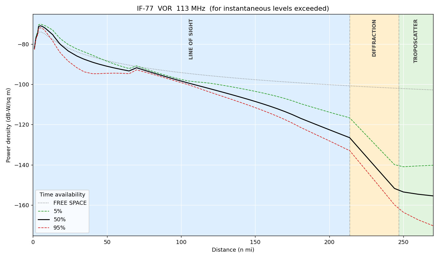
Results of sample input deck provided with IF-77 Fortran version
Background
The IF-77 RF propagation model was developed by NTIA/ITS in response to a need by the FAA. The first version was released in 1973 and then enhanced and a newer one released in 1977. While the Longley-Rice model provides reliable predictions for many ground to ground links, it is unsuitable for use when one or both nodes are at high altitude. The FAA funded Gary D. Gierhart and Mary Ellen Johnson to study the problem and find a solution. The model combines line of sight, diffraction, and tropospheric scatter regions to provide a reliable prediction of link quality. (The model is more recently published as ITU P.2345, "Propagation Model for IF77" though I spotted some errors and seems to be lacking full details on raytracing for implementation.)
More can be learned at the NTIA/ITS IF-77 page, where reports and Fortran software are available.
Download
Download the python code! It is run exactly like the original fortran version. For example,
ata.py < atoa.in
Porting to Python
The original IF-77 development took place on a CDC 6600 which has 60-bit word architecture. The compiler would have been Fortran 63 or more likely Fortran IV. The IF-77 code is challenging to port because of heavy use of GOTOs, often with jumps leaving mid-loop and others re-entering elsewhere. Not impossible, but let's say a tad challenging! I have been unable to find another port, probably in large part due to the very tangled control flow.
The program was first ported as exactly as possible with only changes required by language. For example, slightly needless things are currently retained like pi = 4.0*math.atan(1.0). :-) Change nothing and introduce no bugs!
Enhancement 1
But I didn't take my own advice and made changes. While the program still accepts the original card deck input for those with years of carefully crafted decks, it now also supports a modern config file. The program peeks at the input file and determines which is used. The user need not explicitly specify which. The config.py file can be run directly to see a list of config options and their defaults:config.py --templateSave the template output to a file and edit for your test.
Two equivalent set up files are included as examples: regions.in, the original card deck style, and regions.cfg, the config style input.
Enhancement 2
A second helpful enhancement is the creation of a plot for each case in the input file. The plot at the top of this page is created from the the new style atoa.cfg or atoa.in VOR input deck provided with the original IF-77 years ago. It is interesting to consider the hump at the leftmost portion of the curves. The hump is the VOR’s vertical antenna pattern, not propagation. Card 2 selects facility antenna type 4, the 4-loop array with a cosine vertical pattern. That gain follows the cosine of the elevation angle and drops toward zero straight overhead, the VOR’s "cone of silence". :-) The aircraft is at 30,000 ft, about 8.8 km above the effective surface, so close in that it sits almost directly overhead. EIRP minus spherical spreading plus 20log10(cos elev) is within half a dB of the table’s FREE SPACE column. The curve peaks near 4–5 n mi. Inside that, the rising gain beats the spreading loss. Beyond it, spreading wins and the curve falls normally.
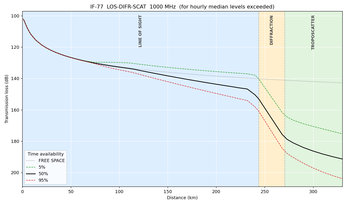
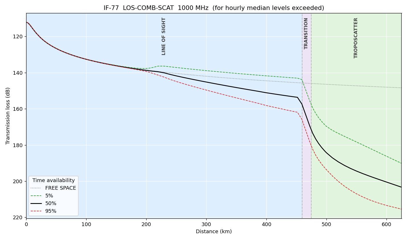
The config below yields the two plots. They show results both at 1 GHz with horizontal polarization, average ground and climate 5. (DIFR is diffraction and COMB is combined diffraction/scatter):
- LOS-DIFR-SCAT: facility at 130 m MSL, aircraft at 3,000 m. Its regions are LOS to 243.8 km, DIFR to about 270 km, then SCAT.
- LOS-COMB-SCAT: facility at 300 m MSL, aircraft at 10,000 m, out to 600 km. Its regions are LOS to 459 km, a narrow COMB band to about 477 km, then SCAT.
The config file:
    case LOS-DIFR-SCAT
    dmax    320

    case LOS-COMB-SCAT
    dmax    600
    hla     300   # Tall facility...
    hai     10000 # ...and high aircraft make scatter line win.
Using IF-77 in Your Programs
As helpful as it is to see that the code does just what the Fortran does, nowadays that is probably not useful and you want to call it in your own programs. Happily, it is easy. A tiny program like this
    import if77

    inputs = dict(f=1000., hla=130., hai=3000., dmax=300., klm=5)
    r = if77.run(**inputs)

    print(r.ok, r.status, len(r.dist), 'rows')
    for i in (0, 40, 60, 81):
        print(r.dist[i], r.levels['50%'][i], r.levels['5%'][i], r.mode[i])
    print('radio horizon (km):', r.horizon['dml_km'])
yields
    True ok 82 rows
       dist_km   50%     5%     95%   mode
         1.00  -102.1  -102.1  -102.1  LOS
       164.67  -140.0  -133.8  -144.3  LOS
       229.60  -146.5  -136.9  -153.8  LOS
       310.00  -188.3  -172.2  -199.8  SCAT
    radio horizon (km): 243.8
More results are returned above in namespace r. I will soon enhance this page by describing the others.
Bugs :-o
Yes, bugs were found in the original Fortran after all these decades. Some are certainly bugs, some are likely and must be investigated but currently all are ported as is:
- DFRAC: IF(K1.LE.00001) - the literal is the integer 1, so test is always true. K_FLOOR in asorp.py (set to 1.0E-5 for probable intent).
- ATA, ENO > 500: ENS=LOG((1.-6370./EFRTH)/.04665) has no /.005577.
- Sea state: report prints state ISS+1, RECPX uses SSH(ISK+1) with ISK=ISS+1, i.e. roughness of next state up.
- KE=0 path: degrees shown come from input IDG, not computed angle.
- COMB always prints its 35 line table (PRINT_COMB_TABLE).
- JB is only set in AALOS. ICPT, BK (in AALOS), KP can be used uninitialized. BK of ATA keeps its value from case to case, as in a Fortran main program.
- MAX1/MIN1 in COMB truncate to integer.
Future
My other web pages show rfl using ITM for link budgets. Eventually, I hope to pull IF-77 into rfl so that altitude will trigger using IF-77. This is firmly in hope category at the moment! :-) The Longley-Rice ITM takes as input an array of distances where loss calculations are wanted. IF-77 takes start and end points and calculates crossovers. It returns the array of distances, so works a little differently from the programmer's standpoint.
Contact
Please get in touch if you spot or fix bugs, or if you have ideas.
Thanks!
-Mike