The repeater transmits 90W (50 dBm) from a 33.5m tower 269m above sea level. In Joe's back yard, he transmits 300W (55 dBm) from a 25m tower 162m above sea level. Predicting power at a receiver is called a 'link budget' and is best accomplished in dB and dBm. Similar to RIAA audio equalization on records, decibels make tiny numbers bigger and big numbers smaller. Best of all, multiplication and division turn into addition and subtraction. A link budget starts with transmit power, then adds all gains and subtracts all losses. Gains are due to antennas, losses from many sources: cable, vswr, insertion losses, noise figure, and the trickiest - path loss.
In 1968, Anita Longley and Phil Rice released software implementing their famous path loss model called Longley-Rice Model or ITM (Irregular Terrain Model). It incorporates a number of sources of loss to predict path loss over terrain. More detail is at https://udel.edu/~mm/itm/ where I share some graphs and biographical info on Longley and Rice as well as ITM code used to study Joe's two transmit situations.
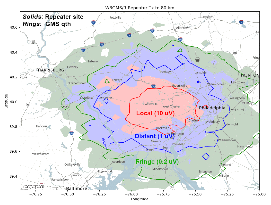
Imagine a 30x30 grid overlaid on a 160km x 160km map centered at the transmit point. A link budget is performed from repeater site or back yard to each grid cell, or 900 link budgets, where each uses ITM. Each link budget is simply:
tx (dBm) + gains (dB) - losses (dB) = rx (dBm)where dBm is decibel relative to a milliwatt and represents real power. Plain old dB is a relative value. For the repeater site, on some path you might have
50 dBm + (5 dBd + 2.15) dBi - 155 dB = -98 dBm, or an S5 signalYou can never add two dBms, but can add or subtract dBs to them. The grid is eventually filled with rx powers and plotted with contours the same way weather maps are. In a laboratory test all gains and losses are carefully measured. In this case, there is a good bit of guess work. What losses does the average ham deal with? Home vs mobile, quality vs budget cable, careful impedance matching of antennas vs compromises, and so on. So take the graphs with a grain of a salt. They represent typical conditions plus or minus 10 dB...or more! The comparisons can be more useful than the absolute numbers. The plot shows three regions: local, distant and fringe. Fringe represents about 0.2 uV or -121 dBm receive power after taking into account noise power, which is itself based on another environmental model. The 'distant' region is where many of us reside, and some lucky few are in the 'local' region.
73!
Mike ab3ap