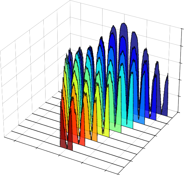
Some eye candy generated by the code below (axis values removed):
Cyclostationary signal processing (CSP) exploits a property of communications signals, periodicity in statistical characteristics, that ordinary spectral analysis misses. It is a powerful tool for signal detection, classification, and parameter estimation in noisy or contested radio environments.
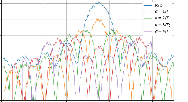
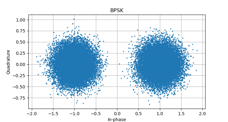
Here is a good example of CSP at work. Imagine two BPSK signals with different symbol rates and slightly different center frequencies. Looking at the combined BPSK signals - created with mksig.py -d, described below - the traditional PSD is unable to discern that two signals are overlapping. CSP, on the other hand, nicely pulls them apart and can provide further details on each. (Signal is from Eric April's 1991 paper, "The Advantages of Cyclostationary Processing." CSP plot by cspPlot.py, below.)
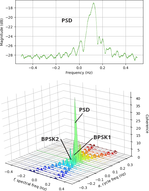
(Code to create 3d SCF slices, above.)
For practicing engineers CSP has felt a bit out of reach until Dr. Chad Spooner created his cyclostationary blog. It is incredibly helpful bridging the gulf between theoretical and practical CSP, especially the trail of posts he put together for CSP beginners. Even at that, I was often challenged to make my code re-create what is presented in the blog. That says more about me than the blog!
I share my python efforts, hopefully useful to fellow students stuck working their ways through the blog. A variety of CSP routines are provided in the libcsp.py library. These are called by a script named 'blog' which steps through a number of blog lessons. While libcsp.py is fairly well written and documented, the blog script is admittedly ugly. It simply makes calls to libcsp and plots results, mimicking a sequence of blog entries whose URLs are printed out.
Another program, csp, is a little different. It does the same things as blog, but instead of plotting to screen the plots are bundled up in a small report. It also steps through the process of blind analysis followed by study of frequencies with highest SCFs. A LaTeX document is created using canned descriptive text including pointers to cyclostationary.blog. If pdflatex exists on your machine, csp will run it and create csp.pdf. If it does not exist, you still have the .tex file and graphs in case you want to run latex on another computer. The expectation is that a CSP-knowledgeable engineer edits and enhances the .tex file to turn raw data into useful information.
In the source code you will occasionally see dead blocks of code. You can delete them, but they were left so that the student is aware of options. Particularly useful is a loop version and vector version of the same SCF subroutine. The loop version is simpler to understand but slower. It can be a stepping stone to understanding the vector version.
These are after hours efforts by a newcomer to CSP, not an expert. Treat this code as best effort from a fellow CSP student, not an answer key from the professor. Please correct, improve and build on what I've started. The files are:
Or download all files in one tar file cspCode.tar.bz2 which will untar into a directory named cspCode.
The code requires python3 as well as the following libraries:
If you want csp to create a pdf you also must install:
On linux, the programs will likely run simply by typing their names. The first python found in your path will be used. If this is not the correct python, use the explicit command:
/path/to/python progwhere prog is one of the python programs described below.
To generate plots from several blog posts, simply type the script name:
blog
Before each plot is presented, a URL to the corresponding blog is printed so you can easily jump to it.
The mksig.py program described below can create a great CSP demo signal from Eric April's 1991 paper, "The Advantages of Cyclostationary Processing." CSP is able to resolve two overlapping BPSK signals that are indistinguishable in a conventional power spectrum, demonstrating the strength of the technique. To create and analyze the overlapping BPSK signals:
where rpt is a directory that will contain many plots and tex files generated by csp. My pdf reader is atril, but replace by whatever you use. The csp program also accepts Matlab 5.0 files as input. So you can similarly do something like:mksig.py -d csp -i bpskDual.iq -o rpt atril rpt/csp.pdf
To see if this is something helpful to you, here is a sample report generated by csp using an 802.11a signal as input.csp -i wifi-802.11a.mat -o rptwifi atril rpt/csp.pdf
You might also want to create the signal used in many cyclostationary.blog articles:
mksig.py -b 0.1 -c 0.05 -n 4000 -s 10 -t bpsk -o bpsk
To generate IQ test signals:
$ mksig.py -h
Usage: mksig.py [-b bps] [-c fc] [-f fs] [-h] [-n n] [-o out]
  [-r] [-s snr] [-t type]

-b: default 0.1, bits/sec.
-c: default 0, center freq in Hz.
-d: dual BPSK example, creates bpskDual.iq and bpskDual.mat.
-f: default 1, sample rate in Hz.
-h: help message.
-n: default 10, number of symbols.
-o: output file name without extension.
-p: default 0, phase noise random intensity.
-r: use square root raised cosine pulse shaping.
-s: default 30, SNR in dB.
-t: default bpsk, type of signal.  Any of
    bpsk, qpsk, 4psk, 8psk, 4qam, 16qam, 64qam.
The program creates two files. One is raw I/Q with a .iq extension, and the other is a Matlab 5.0 file with .mat extension.
If you enhance or debug the code in any manner, please let me know. For that matter, please feel free to drop a line simply to say you find this page useful.
If you have trouble getting the programs to run on a linux box, I'll help
as I'm able. If you have CSP questions, there is a
certain blog
whose author is better equipped to help!