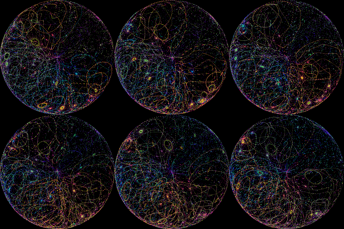
Created with: spirals.py -g spirals.gif -f 100 -N 500
Created with: spirals.py -g spirals.gif -f 100 -N 500
I implemented X user yuruyura's algorithm in a python3 program that you can download and run. It requires pyglet for live animation and PIL for animated gif creation.
pip install pyglet
pip install Pillow
Here are usage options,
$ spirals.py -h
Usage: spirals.py [-h] [-f frames] [-g gifFile] [-k feedback]
           [-m spirals] [-n pts] [-N pixels] [-r rate]
       -h, help message.
       -f int, default 60, GIF mode only: number of frames.
       -g str, if given, animated GIF file name.
       -k float, default 1, feedback intensity.
       -m int, default 250, number of spirals.
       -n int, default 250, points in each spiral.
       -N int, default 400, make N x N image.
       -r float, default 30, Hz frame rate for live or GIF.
       -t int, default 50, speed of evolution, bigger is slower.
Modifying rotation of the complex exponent results in different but still mesmerising movement. Experimentation is recommended!
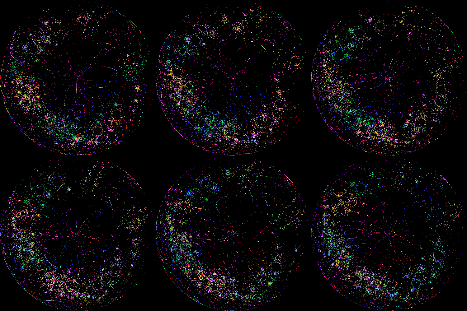
Paul Dunn posted his BASIC conversion of this interesting algorithm on his YouTube page and called it Bubble Universe, in this page's title as well because the original author doesn't name his many creations. It impressed me enough to study it and figure out how it works, a far cry from the creativity to come up with the idea! I'm an engineer, not a mathematician, and offering my best effort at analysis below. Mathematicians, please correct and be gentle. :-)
After converting to complex, I noticed that the equation shares some general similarities with the Burning Ship fractal but that seems to be coincidence. Burning Ship/Mandelbrot-like systems look like \[ z_{n+1} = f(z_n, c) \] and investigate escape behavior. The universe of spirals is instead \[ z_{n+1} = f(z_n) \] and guaranteed to live in a disc of radius 2.
In any case, a few lines of math create a surprisingly complex and attractive animated image. The core of the math is similar to Spirograph style trochoids in that both are created by summing two phasors. Trochoids, however, have a constant angular velocity and Universe, as shown below, has an interesting non-linear feedback mechanism. Shapes are generated, the "bubbles" in Dunn's name, looking like spiral galaxies. Nested for loops are used where the outer loop specifies the number of spirals to create, and the inner loop generates points in each spiral. Simple arithmetic is used to generate RGB values for coloring. The red and green are directly based on the two loop counters, and blue is based on the counters' sum.
Dunn and the original author use real numbers but a complex exponential concisely characterizes a spiral. For example, the following spirals are generated by the expressions shown. Both angle θ and radius r gradually increase from zero. (\(j = \sqrt{-1}\).)
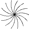
\( r e^{\theta j} \)
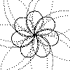
\( r e^{\theta j} + r e^{8\theta j} \)
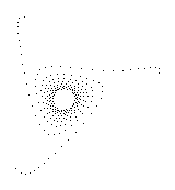
It is more involved with Universe spirals. Well, they are spiral-like objects and I will continue using the slightly incorrect name! For some spiral \( m \) that will contain \( n \) points, its initial phase is \[ \phi_m = t + \frac{2\pi m}{n} \] and initial point \[ z_{m,0} = e^{jm} + e^{j\phi_m} \] Variable \(t\) is incremented by a small \(\Delta t\) at each iteration to generate a new and closely related system, providing the animation. Once a spiral is kicked off with the above, a recurrence provides the next point \( k+1 \), \[ z_{m,k+1} = e^{j(m\ +\ \text{Re}(z_{m\ ,\ k\ }))} + e^{j(\phi_m\ +\ \text{Im}(z_{m\ ,\ k\ }))} \] Here is one after some iterations,
Why does the recurrence equation yield a spiral? First, let's rewrite as \[ e^{aj} + e^{bj} \] which can be rewritten from identities that we never, ever forgot from calculus :-) \[ e^{aj} + e^{bj} = 2\cos\left(\frac{a - b}{2}\right) e^{j(a + b)/2} \] where we note from above that \[\begin{aligned} a &= m + \text{Re}(z_\text{prev}) \\ b &= t + \frac{2\pi m}{n} + \text{Im}(z_\text{prev}) \end{aligned}\] The important things to notice are that both radius and angle are functions of \(a\) and \(b\), and both of those are functions of \(z_\text{prev}\). That is, \[\begin{aligned} r &= 2\cos\left(\frac{a - b}{2}\right) \\ \theta &= \frac{a + b}{2} \end{aligned}\] so the previous \(z\) controls both new radius and new angle, generating the spiral-like set of points. But where does the spiral shape come from? For each spiral, initial phase values are \(a_m = m\) and \(b_m = t + 2\pi m/n\). As \(m\) goes from 0 to \(n-1\), \(2\pi m/n\) rotates through \(2\pi\). So you have \(m\) spirals initialized with different phases making the pretty picture.
Each of those values represents a point on the complex plane which will be plotted using some RGB value. The points are additionally mapped to a larger square image. For example, a 200x200 matrix of complex points might be plotted in a 1000x1000 pixel area. The spreading out of points often enhances the attractiveness of the image.
I work in an RF lab doing a lot of DSP with I/Q (in-phase/quadrature) signals. If you happen to have a similar background you'll find this easy to absorb because it is a feedback phase-modulation system. The derivation that follows is what is implemented in spirals.py and specifically spirals(). Let's start with variables like the analysis above, \[\begin{aligned} \alpha_0 &= m \\ \beta_0 &= \phi_m \end{aligned}\] From them we create two phasors \[\begin{aligned} P_1 &= e^{j\alpha} \\ P_2 &= e^{j\beta} \end{aligned}\] and add them to get \[ Z = P_1 + P_2 = I + jQ \] when we have our old friends I and Q which are used to phase modulate. \[\begin{aligned} \alpha_\text{next} &= m + I \\ \beta_\text{next} &= \phi_m + Q \end{aligned}\]
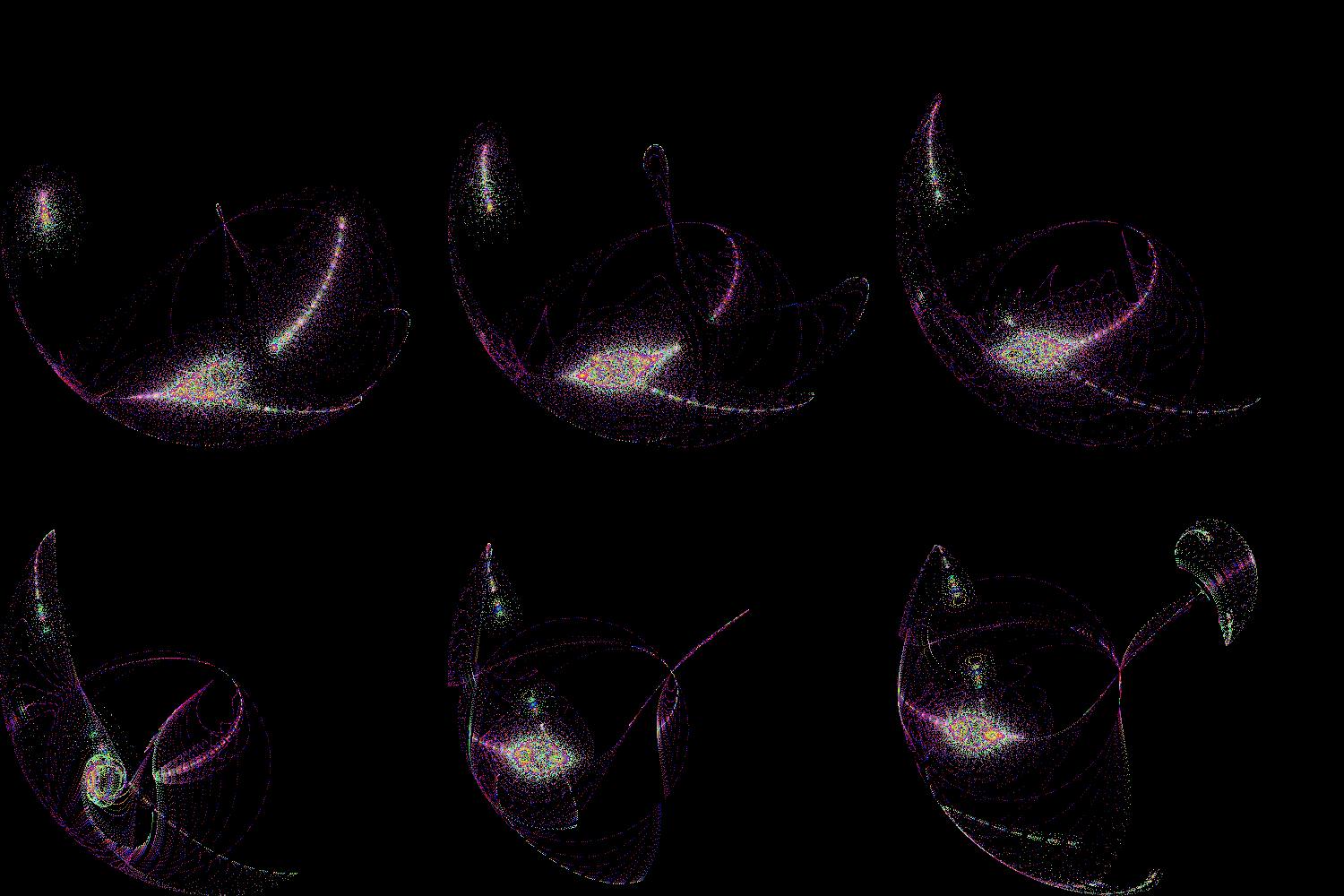
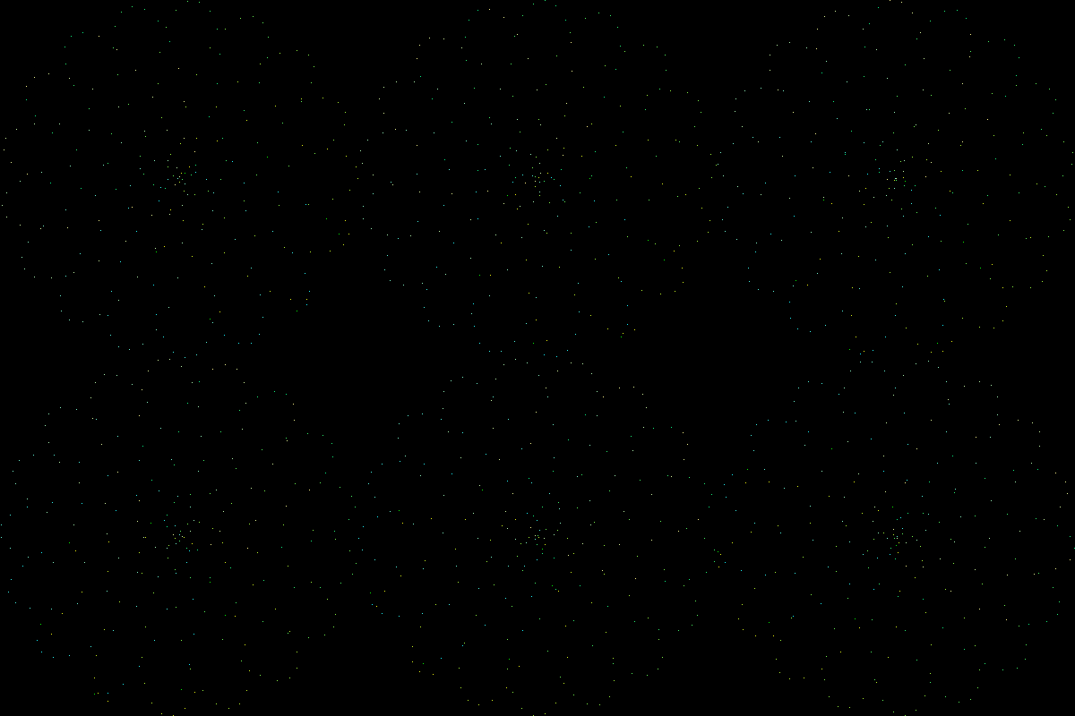
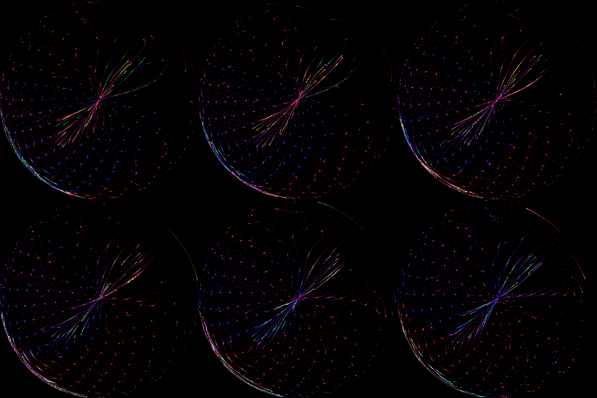
But wait, there's more! Let's provide a way to modify intensity of that feedback, \[\begin{aligned} \alpha_\text{next} &= m + kI \\ \beta_\text{next} &= \phi_m + kQ \end{aligned}\] where k=0 is no feedback, k=1 is the original system, 0<k<1 is weaker feedback, and k>1 is stronger. spirals.py provides the k feedback argument to experiment with. Values near 1 are most interesting, even just a few thousandths away. Here are some examples showing various levels of feedback.
From spirals.py -f 120 -k 0 -g fdbk-0.gif
From spirals.py -f 120 -k 0.75 -g fdbk-0.75.gif
From spirals.py -f 120 -k 1.1 -g fdbk-1.1.gif